An Enhanced Framework for Zero-Shot Reinforcement Learning
Lauriane Teyssier | Advisor: Zhang Ya-Qin
Zero-shot RL aims to build reinforcement learning decision-making agents that,
after exploring an environment without any specific goal, can instantly solve new tasks.
This project, my master thesis, introduces a new algorithmic framework that improves performance by up to 30%,
generalization, and computational efficiency by 50% in this challenging setting.
I'll explain here step by step the thesis problem and proposed contributions.
An Introduction to Reinforcement Learning
Reinforcement Learning is about learning by trial and error—just like humans do.
An agent tries different actions in an environment
and learns over time which decisions lead to the best results or rewards.
- Applications: RL is widely used across several domains:
- Robotics: For learning motor control and adaptive behaviors.
- Autonomous Driving: To train vehicles to navigate complex environments safely.
- Games: Deep Blue (chess, 1997) and AlphaGo (Go, 2016) outperform world champions.
- Large Language Models (LLMs): Used to improve reasoning (e.g., DeepSeek) and align outputs to human preferences and values.
- Advantages: RL allows agents to learn through trial and error by interacting with their environment. It can uncover effective strategies that are too complex to be hand-coded and often exceeds dataset-based approaches by discovering better actions.
Reinforcement Learning pioneers Richard Sutton and Andrew Barto received the 2024 Turing Award.
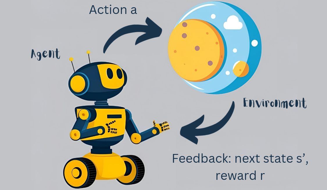
Agent interaction with the environment
Formally, we train an agent to maximize the expected (discounted) reward Q. For a state s, and action a:
$$
Q(s, a) = \mathrm{E} \left[ \sum_{t=0}^{\infty} \gamma^t R_{t+1} | S_0 = s, A_0 = a \right]
$$
with \(\gamma\)
a discount factor
to account that future rewards are more uncertain and less profitable than present ones,
and R the reward.
We then find the best next action function (the policy) \(\pi^*(s)\)
by taking the one that maximizes the expected reward:
$$
\pi(s) = \mathrm{argmax}_a Q(s, a)
$$
RL Challenges:
RL is hard to scale—training requires heavy compute and simulations,
in the contrary to other machine learning fields that scales with large datasets.
Each new task typically requires training from scratch, limiting generalization and broader adoption.
A general and data-efficient RL system would dramatically reduce environmental and financial costs, enabling broader adoption of decision-making agents.
The Zero-Shot RL Problem
The RL community is working toward building agents that can generalize across tasks—that is, agents that can learn to act optimally for any reward function, without needing to be retrained for each one.
At the same time, there's a growing focus on how to leverage datasets to improve performance as more data becomes available, reducing reliance on costly simulated environments.
The challenge of creating flexible agents trained from datasets is known as Zero-Shot Reinforcement Learning.
Solving the Zero-Shot RL Problem:
Instead of teaching the agent which actions to take for a specific reward during training, we focus on helping it understand how the environment works. At inference time, the agent combines this knowledge with the reward function to compute the best strategy. Imagine a robot that freely explores a room without instructions, and then—on its first try—is able to fetch an object or avoid obstacles when asked.
Instead of teaching the agent which actions to take for a specific reward during training, we focus on helping it understand how the environment works. At inference time, the agent combines this knowledge with the reward function to compute the best strategy. Imagine a robot that freely explores a room without instructions, and then—on its first try—is able to fetch an object or avoid obstacles when asked.
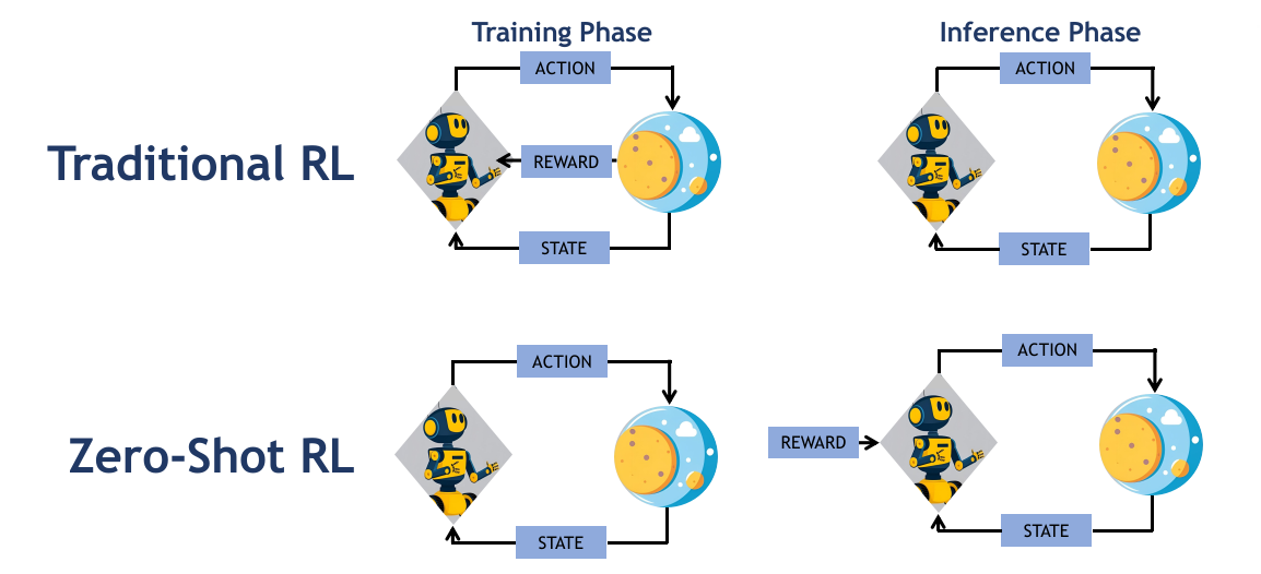
Agent generalizing to new tasks
Current Methods Limitations:
Our Goal:
Address all three challenges by building on a current state of the art, FB Representations, and developing a method that improves performance, reduces computational time, generalizes more effectively across diverse tasks.
- Low performance — especially when methods rely on human-designed assumptions
- Poor generalization — current solutions only work in simple environments with high-quality data
- High computational cost — most approaches are resource-intensive
Our Goal:
Address all three challenges by building on a current state of the art, FB Representations, and developing a method that improves performance, reduces computational time, generalizes more effectively across diverse tasks.
State-Of-The-Art: Forward-Backward Representations
Forward-Backward Representations:
Instead of directly learning the expected discounted reward Q,
the FB Representation approach focuses on learning the expected discounted state-action visitation probabilities M,
which are less dependent on the reward.
These two quantities are related by: \(Q = M \cdot R\).
To learn M, we use its Bellman equation—similar to Q-learning—describing how the visitation probabilities evolve:
\[
M^{\pi} =
\underbrace{P}_{\text{Direct transitions from } (s,a)}
+
\underbrace{\gamma P_{\pi} M^{\pi}}_{\text{Future transitions arriving at } (s,a) \text{ from others}}
\]
Here, \(P\) represents the transition probabilities and \(\gamma\) the discount factor.
We turn this Bellman consistency into a learning objective:

\[ \mathcal{L}(M) = \mathbb{E} \left[ \left\| M^{\pi}(s_0, a_0, ds, da) - P + \gamma P_{\pi} M^{\pi}(s, a) \right\|^2 \right] \]
However, learning M directly is too difficult (intractable) due to its complexity.
To simplify, we use a low-rank decomposition:
Using this equation solely is not enough to learn M, as M is too complex to be learned directly.
\[M^{\pi^z}(s_0, a_0, ds, da) = F(s_0, a_0, z)^{\top} B(s, a)\].
Here, \(z\)
is a latent representation of the reward function—meaning it’s a compact,
hidden encoding of the reward that the model can use as input to the function F,
and later to compute the final policy.
It is computed as: \[ z_r = \mathbb{E}_{s \sim \rho}[r(s) B(s)] \]
In this formulation, \(B(s, a)\) captures environment dynamics (the next-state/action dependency of M),
and \(F(s_0, a_0, z)\) encodes the initial state-action and task embedding.
The new objective with this decomposition becomes:
$$
\begin{aligned}
\mathrm{L}(F, B) = & \|F_z^{\top} B\rho - (P + \gamma P_{\pi_z} F_z^{\top} B\rho)\|_{\rho}^2\\
= & \mathrm{E}_{(s_t,a_t,s_{t+1})\sim\rho, s'\sim\rho}\left[\left(F(s_t, a_t, z)^{\top}B(s') - \gamma \bar{F}(s_{t+1}, \pi_z(s_{t+1}), z)^{\top}\bar{B}(s')\right)^2\right]\\
& - 2\mathrm{E}_{(s_t,a_t,s_{t+1})\sim\rho}\left[F(s_t, a_t, z)^{\top}B(s_{t+1})\right] + \text{Const}\\
\end{aligned}
$$
Finally, the optimal policy is obtained by selecting the action that maximizes the expected reward:
$$
\begin{aligned}
\pi^R(s) = & \mathrm{argmax}_a Q(s, a) \\
= & \mathrm{argmax}_a \sum_{s_0, a_0} M^R(s_0, a_0, s, a) \cdot R(s,a) \\
= & \mathrm{argmax}_a \sum_{s_0, a_0} F(s_0, a_0, z_R)^{\top} B(s, a) \cdot R(s,a)
\end{aligned}
$$
Main issues with existing the FB learning methods:
- Performance: The original model uses simple MLP architectures of 3 layers maximum. These are not powerful enough to handle complex patterns. Moreover, simply increasing the size of the networks (i.e., adding more parameters) does not lead to better performance. In fact, it makes training harder without effectively capturing the more complex patterns found in richer datasets or more difficult problems.
- Distributional Shift: If the dataset does not include the action \(\pi(s_{t+1})\), the algorithm receives no feedback to correct its prediction at that point. As a result, it may assign unrealistic values to \(\pi(s_{t+1})\), which leads to biased training.
FB limitations
Summary of Our Contributions
To address the limitations of the current FB method, we introduce a series of improvements targeting both algorithm design and training efficiency:
- Better FB Algorithm: We improve the learning process by adding a regularization term, which makes learning more stable and generalizable.
- Upgraded Neural Networks: We replace basic MLPs with transformers, which are better at capturing complex relationships in the data.
- Faster Training: Thanks to these changes and code optimizations, we reduce training time from 17 hours to just 11 hours on a single A8000 GPU.
Our Neural Network Improvements
Switching from MLPs to Transformers offers several advantages:
- Understanding sequential relationships: For learning the function \(B\), which captures how actions follow states, the task is similar to understanding word order in a sentence—something transformers excel at thanks to their success in natural language processing.
- Flexible input interactions via attention: The function \(F\) takes action, observation, and reward representation (\(z\)) as input. Attention layers allow the model to learn complex interactions between these inputs.
- Improved generalization: Transformers have been shown to generalize better than MLPs, especially in settings with high complexity or rich data distributions.
- Future-proof architecture: Transformers are a highly active area of research, with ongoing work focused on reducing their computational cost. By adopting this architecture, our model can easily benefit from future improvements in transformer efficiency and scalability.
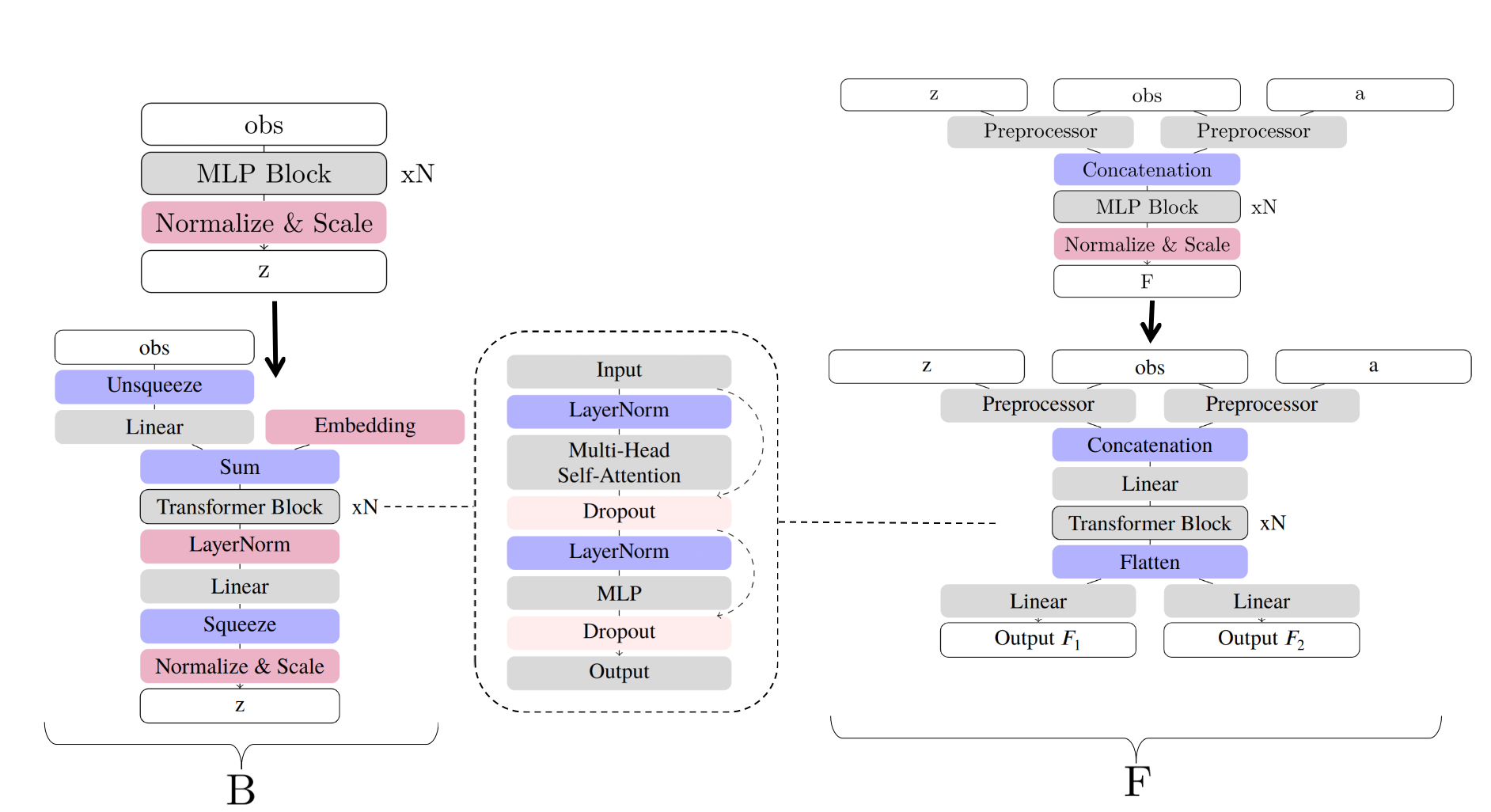
Schematic description of the neural network changes
Our Regularization Scheme
To make training more stable, we introduce a regularization technique that helps avoid learning from states that might be overestimated.
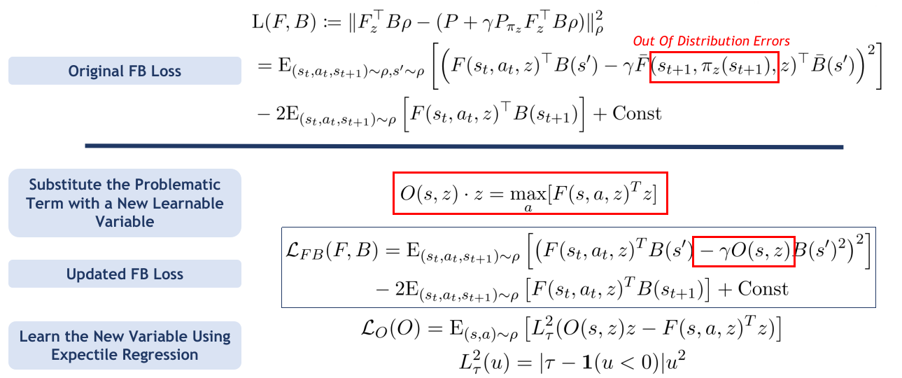
Instead of directly using the potentially inaccurate term \(F(s_{t+1}, \pi(s_{t+1}), z)\), we introduce a new variable \(O\), defined as: \(O(s, z) \cdot z = \max_a [F(s, a, z)^T z]\). This acts as a safe substitute, replicating the behavior of \(F\) while avoiding its overestimations.
But how do we learn this new variable \(O\)? We want it to behave like \(F\), but only where \(F\) isn’t overconfident. So we train \(O\) to match only the lower 70% of \(F\)’s outputs, ignoring the potentially overestimated top 30%.
This training method is called expectile regression: instead of learning to copy the average output, the model learns to match a target percentile of another model’s values.
Once trained, using \(O\) in place of \(F\) in the loss function helps us avoid instability and leads to more robust learning.
Our regularization scheme step by step
Our Computation Speed Improvements
We applied several optimizations to make training faster without hurting performance.
By profiling the code, we found and fixed slow parts.
We used
bfloat16 precision (where possible) to speed up training, and enabled torch.compile to optimize runtime execution.
On supported GPUs, we used TF32 for fast matrix operations with minimal accuracy loss.
These changes brought up to 10× speed improvements, depending on the setup.
| Optimization | Speedup | Notes |
|---|---|---|
| Baseline | 1× | Standard training, no optimization |
torch.compile |
2× | Just-in-time model graph optimization |
| TF32 Matrix Ops | 5× | Fast GPU matrix multiplications |
bfloat16 |
10× | Faster training, used without regularization |
Experiments & Results
- Benchmarks: DeepMind Control Suite (Quadruped, Point Mass Maze, Walker)
- Findings: Our method (FB-PERL, orange) presents 9%–34% IQM (Interquartile Mean) improvement over previous state-of-the-art, faster training and better generalization.
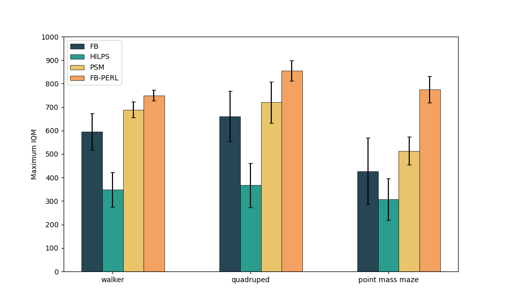
Performance graphs
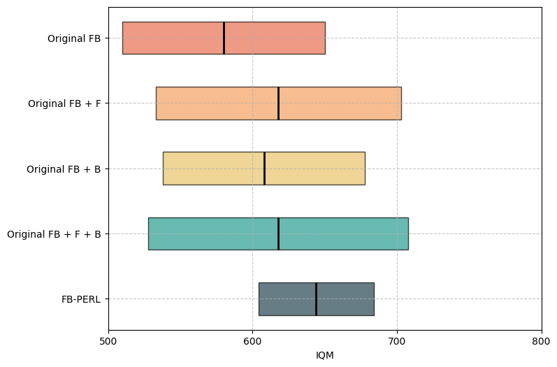
Ablation study results
Conclusion & Perspectives
This thesis advances zero-shot RL with a more expressive, robust, and efficient framework.
While progress is significant, challenges remain in scaling to even more diverse tasks and improving robustness to low-quality data.
For more technical details, please refer to the full thesis report linked below.